

By Carola F. Berger, PhD, Dipl.-Ing., CT
For the readers who have been wondering whether I have made any progress with my neural machine translation project, indeed, I have. I have successfully installed and run OpenNMT with the default settings as in the tutorial, though the resulting translations were fairly terrible. This was to be expected, since a whole lot of fine-tuning and high-quality training corpora are necessary in order to obtain a translation engine of reasonable quality. However, as a proof of concept, I am fairly impressed with the results. As the next step, I am planning on tinkering with the various individual components of the NMT engine itself as well as the training corpus to improve the translation quality, as much as one can without some major programming work. Before going into all the gory details in future blog posts, let’s first have a look at a relatively simple artificial neural network. I presented this example at the 58th Annual ATA Conference, the full slide set can be found here.
Neurons and Units
In the following, unless explicitly stated otherwise, the term “neural network” refers to artificial neural networks (ANNs), as opposed to biological neural networks.
ANNs are not a new idea. The idea has been floating around since the 1940s, when researchers first attempted to create artificial models of the human brain. However, back then, computers were the size of whole rooms and consisted of fragile vacuum tubes. Only in the last decade or so have computers become small and powerful enough to put these ideas into practice.
Like biological brains, which are composed of neurons, ANNs are composed of individual artificial neurons, called units. Their function is similar to biological neurons, as shown in the figures below. Figure 1 shows a biological neuron, whose precise function is very complicated. Loosely speaking, the neuron consists of a cell body, dendrites, and an axon. The neuron receives input signals via the dendrites. When these input signals reach a certain threshold, an electrochemical process takes place in the nucleus, and the neuron transmits an output signal via the axon.
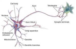
Fig. 1: Biological neuron. Source: Bruce Blaus, https://commons.wikimedia.org/wiki/File:Blausen_0657_MultipolarNeuron.png
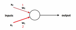
Fig. 2: Unit in artificial neural net
Figure 2 shows a model of a very simple artificial unit. It also receives inputs (labeled X1 and X2), and an activation function (the white blob in Fig. 2) transmits an output signal according to the inputs. The activation function can be a simple threshold function. That is, the unit is off until the sum of the input signals reaches a certain threshold, and then it transmits an on signal when the sum of the inputs exceeds the threshold. However, the activation function can also be much more complicated. As described, this artificial unit does not perform any particularly interesting functions. Interesting functions can be achieved by weighting the inputs differently according to their importance. An artificial neural net “learns” by adjusting the weights (labeled W1 and W2 in Figure 2), or the importance, of the input signals into each unit according to some automated algorithm. In Figure 2, input X1 is twice as important as input X2, as illustrated by the relative thickness of the input arrows.
Layers and Networks
Like biological brains, these units are assembled into a neural network, as shown in Figure 3. More precisely, the figure shows a so-called feed-forward neural net.
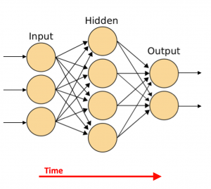
Fig. 3: Artificial neural network. Adapted from: Cburnett, https://commons.wikimedia.org/wiki/File:Artificial_neural_network.svg
ANNs consist generally of an input layer, one or more hidden layers, and an output layer. Each layer consists of one or more of the units described above. Neural networks with more than one hidden layer are called “deep” neural nets. Each unit is connected with one or more other units (indicated by the arrows in Fig. 3), and each connection is given more or less importance through an associated weight. In a feed-forward neural net, as shown in Figure 3, a unit in a specific layer is only connected to units in the next layer, not with units within the same layer or in a previous layer, whereby the terms “next” and “previous” refer to sequences in time. In Figure 3, the arrow of time flows from left to right. There are also so-called recurrent and convolutional neural networks, where the connections are more complicated. However, the main idea is the same. The middle layer in Figure 3 is hidden because it does not have direct connections to inputs or outputs, whereas the input and output layers communicate directly with the external world.
Training and Learning
The thus assembled neural network “learns” by adjusting the various weights, for example, numbers between -1.0 and +1.0, but other values are of course possible. The weights are adjusted according to a specific training algorithm.
The training of a neural network typically proceeds as follows: A set of inputs is fed into the input layer of the neural network. Then, the neural network feeds that input through the network, in accordance with the weights (connections) and the activation functions. The final output at the output layer is then compared to the desired output according to a specific metric. Finally, the weights throughout the network are adjusted depending on the difference between the actual output and the desired output as measured by the chosen metric. Then the entire process is repeated, usually many thousands or millions of times, until the output is satisfactory. There are many possible algorithms to adjust the weights, but a description of these algorithms goes beyond the scope of this article.
An Example
As a concrete example, let’s look at a fairly simple neural network that recognizes handwritten digits. A sample of the inputs is shown in Fig. 4. I programmed this simple feed-forward neural net for Andrew Ng’s excellent introductory course on machine learning, which I highly recommend.
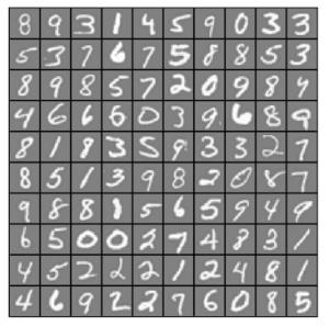
Fig. 4: Sample handwritten digits
The architecture of the neural network is exactly as shown in Figure 3, with 400 input units, since the input picture files have a size of 20 x 20 grayscale pixels (=400 pixels). There are 25 units in the hidden layer, and 10 output units, one for each digit from 0 to 9. This means that there are 10,000 connections (weights) between the input layer and the hidden layer (400 x 25) and 250 connections between the hidden layer and the output layer (25 x 10). In other words, we have 10,250 total parameters! For the technically interested, the activation function is here a simple sigmoid.
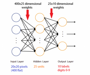
Fig. 5: ANN for handwritten digit recognition
The training proceeded exactly as described above. I fed in batches of several thousand 20×20 labeled grayscale images as shown in Fig. 4 and trained the net by an algorithm called backpropagation, which adjusted the weights according to how far the output was from the desired label from 0 to 9. The result was remarkable, especially considering that there were only a couple dozen lines of code.
But How Does It Work?
The fact that it works is remarkable and also somewhat unsettling, because all I did was program the activation function, specify how many units are in each layer and how the layers are connected, specify the metric and the backpropagation, and the neural net did all the rest. So, how does this really work?

Autopsy of a neural network (Image: Public domain)
To be honest, even after doing some complicated probabilistic and statistical ensemble calculations, I still did not understand how these fairly simple layers of units with fairly straightforward connections could possibly manage to discern handwritten digits. So I went on to “dissect” the above neural net layer by layer, and pixel by pixel. Here’s what is actually happening to the input, after successfully training the neural net.
The first set of weights between the input layer and the hidden layer can be thought of as a set of filters, which essentially filter out important patterns or features. If one plots only this first set of weights, one can visualize a set of 25 “filters,” as shown in Figure 6. These filters map the input onto the 25 hidden units in the hidden layer. Figure 7 shows what happens if you map a specific input, in this case a handwritten “0,” onto the hidden layer.
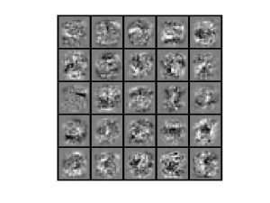
Fig. 6: First set of weights, acting as a “filter”
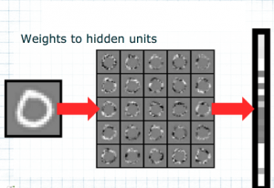
Fig. 7: Mapping of 0 to hidden units
The output of the hidden layer is then piped through another filter, as shown in Figure 8A, and mapped onto the final output layer via this filter/set of weights. Figure 8A shows how the input picture with the digit “0” is correctly mapped onto the output unit for the digit “0” (at the bottom, because the program displays things vertically from 1 at the top to 9 and then to 0 at the bottom).
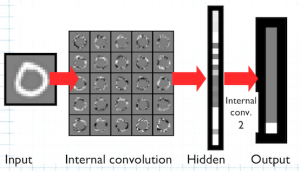
Fig. 8A: Mapping of input to output via hidden layer, handwritten “0”
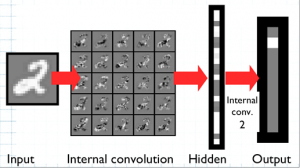
Fig. 8B: Mapping of input to output via hidden layer, handwritten “2”
More examples of this filtering or mapping via the internal sets of weights are given in my slide set for ATA58.
Again, the internal weights act as a sort of filter to pick out the features of interest. Naively, I would have expected that these features or patterns of interest should correspond to vertical and horizontal lines, for example in the digits 1, 4, or 7, or to various arcs and circles, in digits such as 3, 8, or 0. However, this is evidently not at all how the network picks out digits, as can be seen from the visualization of the first set of weights in Figure 6. The patterns and structures that the neural net filters out are ostensibly much more complex than simple lines or arcs. This is also the reason for the “detour” via the hidden layer. A direct mapping from input to output, even with an internal convolution, would not be sufficient to pick out all the information that is necessary to distinguish one character from another. Similarly, for more complex tasks, more than one hidden layer will be needed. The number of hidden layers and units as well as their connections/weights grows with the complexity of the task.
Summary
This blog post aimed to explain the inner workings of a simple neural net by visualizing the internal process. Neural networks for other applications, including for machine translation, work pretty much the same way. Of course, most of these will have more than one hidden layer, possibly pre- and post-processing of input and output data, more sophisticated activation functions, and a more complicated architecture such as recurrent neural nets or convolutional neural nets. However, the basic idea remains the same: The underlying function of an artificial neural net is simply pattern recognition. Not more, not less. While well-trained ANNs are extraordinary and unquestionably better than humans at the pattern recognition tasks for which they are trained because they don’t get tired or have lapses of concentration, one should never forget that they are remarkably ill-suited for anything that goes beyond the tasks they are trained for. In such cases they can sometimes detect patterns that are not there, and sometimes the tasks simply cannot be cast into a pattern, however complicated the pattern might be. In other words, while ANNs certainly exceed their programming, they can never exceed their training (at least until the so-called technological singularity is upon us).
All images created by Carola F. Berger except where otherwise credited.

Carola F. Berger is an ATA-certified English>German patent translator with a PhD in physics and a master’s degree in engineering physics. She became interested in the topic of artificial intelligence after reading about the allegedly impending robot apocalypse. To prepare for the uprising of intelligent machines, or, more likely, for short-circuited self-driving lawn mowers, she has completed several online courses on artificial intelligence and machine learning. She has also constructed an autonomously navigating robot nicknamed Boticelli.